As the market for computing at the edge continues to develop, it will be important for designers to make a distinction between edge systems and endpoint productss. Edge systems are apt to be fairly complex, while endpoints will tend to be simpler, perhaps as simple as a single sensor with ASIC. Whether creating an edge system or an endpoint, designers will almost certainly have the option to use components that provide plenty of operational overhead at a completely reasonable upfront cost. In the first of this two-part series, we’re going to explain why it’s a mistake to let the cost analysis end there; in the second we’ll discuss some developments that may help avoid the problem.
It can seem cheap and easy to build a system with computational and resource headroom beyond requirements, but when it comes to an edge device or an endpoint, it is wise to also calculate size, weight and power / cost (SWaP-C). At the edge, overprovisioning could compromise the SWaP-C of the system, but at the endpoint, overprovisioning can be catastrophic from the standpoint of SWaP-C.
Video cameras are a good starting point as we examine the situation.
Video cameras are ubiquitous. They’re in laptops, game machines, tablets, security systems, smart home appliances, and every smartphone has at least two. There are already many times more cameras on Earth than there are people, and according to LDV Capital, by 2022 there will be 45 billion video cameras in operation. In 2019 over 500 hours of video was uploaded to YouTube each minute of every day. That’s 30,000 hours of video per hour — and YouTube represents only a small part of the video captured each day. Humans cannot possibly watch all the video produced, but then again much of the video captured was never intended to be watched by human eyes, but rather is recorded and archived for future retrieval, or to be automatically analyzed by signal processing and AI algorithms. There’s a potentially huge market serving the AI needs created. But what are the configurations and scenarios of interest?
A common scenario involves monitoring of a scene with multiple cameras / sensors looking for anomalous occurrences such as unauthorized intruders or in a similar usage, using this information from multiple cameras/sensors for vehicle navigation.
Video Usage
For some scene security applications, surveillance video is simply archived and only reviewed if some anomalous event occurs. In other security applications, continuous realtime monitoring of multiple video cameras must be performed. Because it is tedious, and must be monitored continuously, these applications are increasingly turning to autonomous monitoring using Artificial Intelligence (”AI”) systems for video scene monitoring. AI doesn’t have the shortcoming of human monitors who may become distracted, sleepy, may call in sick etc.
In other applications video alone or is augmented with other sensor data and used for vehicle navigation. In this rather demanding application, accuracy, latency and reliability are of critical importance: lives depend on it working properly all the time. Because milliseconds of latency can be the deciding factor in avoiding a collision, analysis of the video & fused sensor data field is generally done locally. Wireless data links are not available at all times and even if available, latency to a cloud-based server may be on the order of seconds, depending on the variability of demand loading. Finally, cloud-based analysis and storage can be expensive vs doing the analysis locally at near-zero cost.
For local processing of an imaging system’s data, there are two basic architectural approaches: collecting and processing/analyzing the sensor data on a common computer, so-called “edge processing”, or distributing the processing resources much closer to each sensor for localized “endpoint processing”. The approach chosen can have a big impact on the SWaP-C of the system as well as its scalability and prospects for future miniaturization.
Edge processing
Edge processing architectures usually are based on a general-purpose reprogrammable media processing computer that includes a collection of sensor input ports and network connections. The media computer will have substantial processing capacity provided by a high bandwidth media processor and will run an operating system such as Linux.
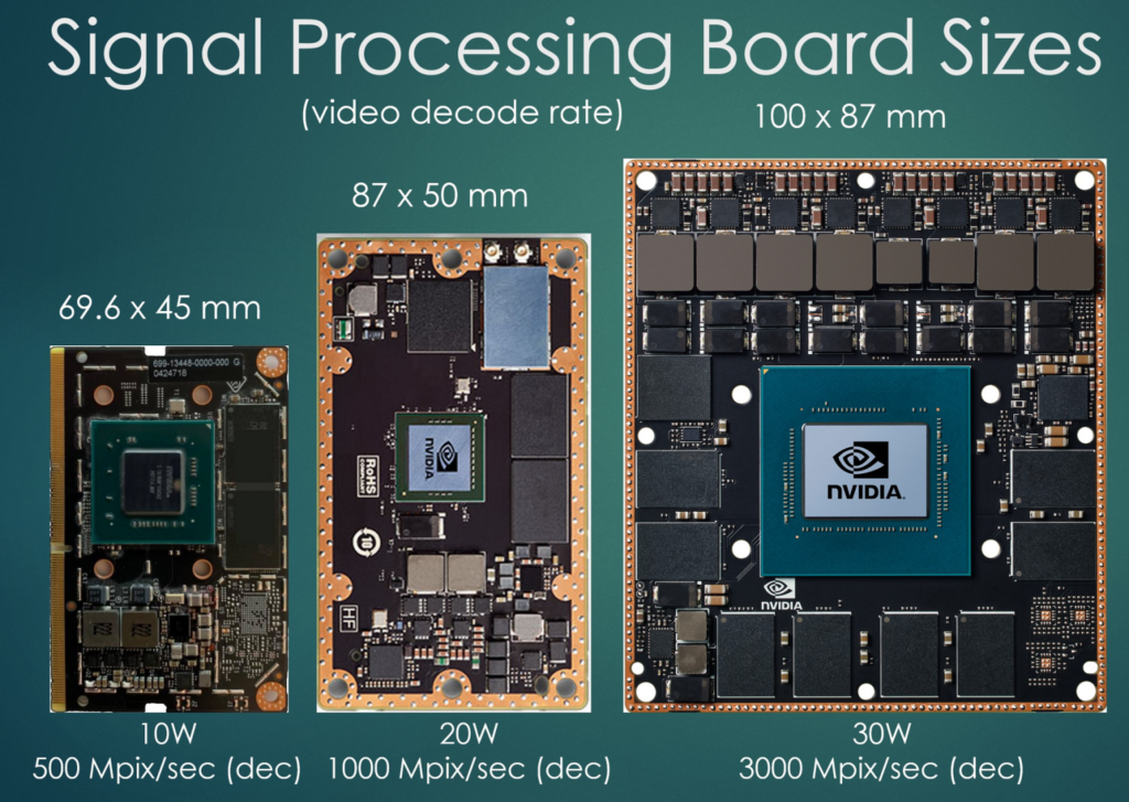
Usually these computers have many gigabytes of high bandwidth DRAM. Because it is a general-purpose media processor, it is designed to efficiently run different workloads. Some are more RAM and processing intensive than others but the computer is designed to offer computational headroom under worst case conditions. An example of three popular signal processing computer motherboards is shown in Figure 1. They differ in size, power and pixel processing performance.
Adding more sensors to such a system may not demand any more processing performance, depending on how close to saturation the design is. However, this excess capability may be costing power and creating thermal issues that are unnecessary in all but a few configurations.
Endpoint processing
Instead of using a common media processing computer, endpoint processing moves high bandwidth media processing to the sensor or to a group of sensors in close physical proximity. In one example an Endpoint Processor node may be a module containing an FPGA and DRAM that connects directly to two or more video image sensors via MIPI ports. The FPGA is loaded with a bitstream that performs a specific function such as object recognition/classification or image quality adjustment and lens distortion correction/image rotation to name two of nearly limitless possibilities. Each node supports a sensor or group of related sensors and each node may have a different task it performs.
In this Endpoint Processing scheme, the first level of processing is high bandwidth data processing / data reduction and is done close to the sensor. The output from the node can be low bandwidth analyzed data vastly reducing the bulk of the data set that is subsequently analyzed upstream. For example, the output of the node could be an indicator that something has moved in the scene and a preliminary classification of what the object is. This can be sent to a nearby processor along with the outputs from other nodes to infer what the overall system is observing by analyzing these preprocessed data streams. In this scenario this nearby processor replaces the high-performance media edge processor of the previous architecture with a simpler and lower power processor that operates on vastly reduced preprocessed data, yet the distributed system yields the same overall result. Variants of the system requiring more or higher resolution / frame rate sensors can be supported by adding nodes or by scaling the nodes to higher performance hardware in accordance with need. The distributed architecture is well-suited for modularized expansion/upgrades.
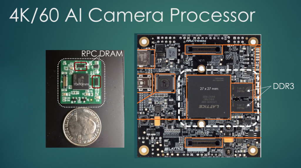
Two implementations of an FPGA plus DRAM processing node capable of 4K/60 AI video are shown in Figure 2. The right side shows conventional BGA packaged Lattice ECP5 Family FPGA and DDR3 DRAM while the left side shows wafer scale packaged components: the DRAM in Fan-in WLCSP while the ECP5 FPGA is in a Fan-Out WLCSP. The entire module on the left is about the same size as the conventional BGA type FPGA package alone on the right. The WLCSP DRAMs are about the size of a grain of rice but are 256 Mbit capacity with the same bandwidth as x16 DDR3. The WLCSP-based node on the left dissipates approximately 1 Watt for the ECP5 FPGA plus 2 DRAMs running a 4K video workload.
SWaP-C Optimization
From a development perspective, it is attractive to use a standard off the shelf media computer in the Edge Processing architecture: the hardware is already designed. Using it can be as simple is cabling up the cameras and sensors to it and then focusing on software development using standard tools running under a standard OS. But is this a power and or space optimized solution? Is it the cheapest solution for a mass market device?
One can look at the “headroom” offered by the hardware as “overprovisioning”: that is to say, you are providing more hardware capability than is needed by the application. There are costs associated with overprovisioning.
Overprovisioning Cost
Besides actual hardware cost, overprovisioning costs can also be observed in power dissipation and physical size (XYZ + weight) of the hardware. Depending on the application, these can be critical deciding factors. For example, a navigation system for a car doesn’t have the same weight, size and power dissipation constraints as does a navigation system for a moderate payload class drone but has many similar requirements for the navigation system in terms of threat detection and collision avoidance and usually has additional degrees of freedom of motion (Z as well as X and Y).
Common ways overprovisioning can enter into a design are the processor and memory silicon: the processor may be more capable /faster than needed. For memory because of a bandwidth requirement and standard memory organizations and capacities, there may be many more memory bits than are actually required by the application and these excess bits consume unnecessary power. An example of the memory bit/bandwidth problem is a 4K/60 video frame buffer. For 24-bit video only 200 mbits is needed but the bandwidth demands DDR3 performance. The minimum capacity is 1 Gbit for JEDEC Standard DDR3 devices. So, using DDR3 is overprovisioning the memory bits by at least 500%: 1 Gbit is 5x the bits needed and was selected only on the basis of bandwidth. A balanced memory would provide the right bandwidth from the correct number of bits to minimize overall power use.
Hidden Cost of Power
Power is an especially sensitive parameter as its cost can manifest itself in different ways that may appear hidden. One is the power supply requirements: higher power means a larger capacity battery for the same runtime in battery powered devices. Larger battery capacity usually means larger physical size, weight and cost. Frequently the size of a device’s housing is set by the battery, so minimizing consumed energy can be very important in some products. making a housing smaller means less materials used and that affects cost.
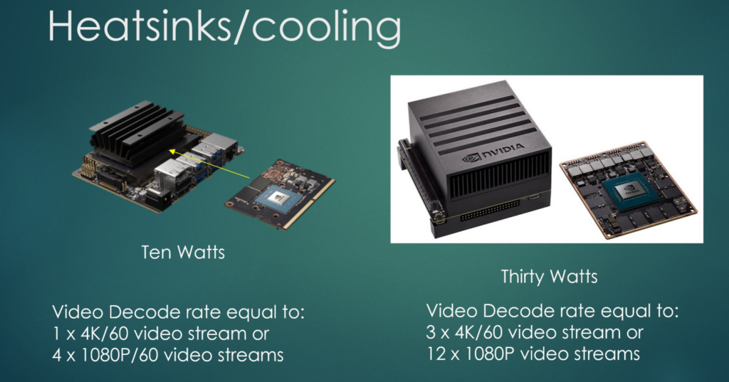
The other way power drives cost is in thermal considerations. A well designed BGA and PCB can usually tolerate up to about 1 Watt without a heatsink, relying on heat conduction into the PCB via solder balls and convection via the package surface to shed the heat. Once a product-specific power dissipation threshold is reached, heatsinks must be used. A higher power dissipation threshold will dictate airflow, ie a fan to be added and so on.
Examples of two of the systems of Figure 1 deployed with heatsinks is shown in Figure 3. One must factor the cooling system for boards that dissipate as little as 5 to 10 Watts. For many applications the XYZ + weight of the thermal solution far exceeds the processor board it is designed to support.
Memory impact on endpoint node
In the next installment, the differences in memory components and how they affect the SWaP-C of the Endpoint Processing Node will be examined and a new high bandwidth memory architecture, optimized for small form factor video applications, will be introduced.
— Richard Crisp is vice president & chief scientist for imaging and memory product development at Etron Technology America
Source: https://www.eetimes.com/realtime-video-swap-c-tradeoffs-for-edge-vs-endpoint-part-1/